Deep learning for computer vision
Ch 5 in Deep Learning with Python (DLP) covers the topic of computer vision. It teaches us how to build DL models that can classify pictures as cats or dogs. You can find my Python code and output here.
Baseline Models and Regularization
For computer vision applications, we use a specific type of DL model called convolutional neural networks (or convnets). Our 1st model clearly suffers the overfitting problem based on the loss and accuracy plots.
As discussed in the last post, we can use regularization such as dropout to mitigate the issue. Therefore, our 2nd model incorporates dropout at the first layer of our classifier.
Also, we introduce a new regularization method called data augmentation. As shown in the four dog images, we apply some random changes to the original image. The transformed (or augmented) images still look realistic enough. We then use the augmented images, together with the original one, as the inputs to train our model.
After the above two regularization methods, the loss and accuracy plots of our 2nd model no longer show severe overfitting.
Visualize Intermediate Convnet Outputs
We can visualize the features that were learnt at each convnet layer of our 2nd model. Here, we picked a picture of a cat face. Notice the features become more abstract and less visually interpretable as we move from lower to top layers. This shows the computer learning process, which is similar to how humans learn. It starts with a concrete and visually describable patterns (e.g., cat eyes and ears) to increasingly complex and visually abstract concepts (e.g., cat).
Use Pre-Trained Convent
Convents for image classification usually consist of two parts: a series of convolutional layers as the base and a densely connected classifier as the top. Therefore, to further improve our model performance, one technique is to use a pre-trained convent base. This reduces training time and is helpful for a small dataset. There are two ways to implement it: feature extraction and fine tuning.
For feature extraction, we first feed our input images through the convolutional base of the pre-trained convnet without updating the weights of the base. Then use the output from the base to train our classifier top (aka update the weights of the top).
For fine tuning, we first feed our input images through the convolutional base of the pre-trained convnet without updating its weights. Then use the output from the base to train our classifier top. Afterwards, we unfreeze some layers of the base and jointly train these layers and our classifier top.
Notice we didn’t start with a fresh model under Approach 5. This is because in Approach 4, we trained our classifier top while freezing the weights of the convolutional base. Thus, Approach 4 effectively completes the 1st step of Approach 5.
Visualize Convnet Filters
Earlier, we visualized how a convnet transforms an input image (e.g., a picture of a cat face) through one layer after another. It shows how computer gradually learns the concept of cat. Now, we visualize the filters used in each layer that are most conducive to learning.
The technique for this visualization task is to use gradient ascent (move the input in the same direction of the gradient). From an earlier post, we know DL models update weights of each layer by using stochastic gradient descent (move the input in the opposite direction of the gradient). SGD intends to minimize a loss function. However, gradient ascent does the exact opposite: it maximizes the loss function and thus showing the filter that is most conducive to learning.
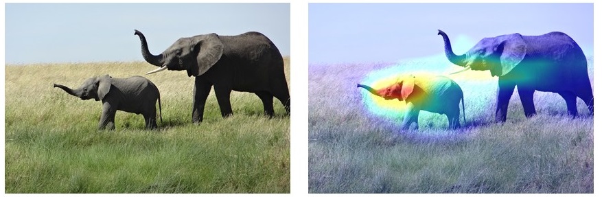
Heatmap of Class Activation
Lastly, we can use a heatmap to identify which parts of an image is most important at helping computer reach the final classification decision. For example, the left image below is the original image. The DL model we used identifies the animals as most likely to be African elephants. The right image shows the heatmap we generated, indicating the ears of the elephant calf plays the most decisive role in this classification. You can find my Python code on generating the heatmap here.